



This post was co-authored by Mal Graham.
Executive Summary
Animal advocates sometimes make claims like “there are X of this animal, and Y>X of this animal, so Y might be a better target to focus on.”
For example, you could imagine someone making a claim like “there are 20 quadrillion ants, so they are a higher priority to work on than Pacific salmon (wild population size: ~500M), even accounting for moral weight and welfare range.”
Some arguments for working on farmed over companion, or wild over farmed animals, take this shape – where population size serves as a rough heuristic for prioritization.
These claims frequently rely on abundance estimates produced by conservation- and evolution-focused scientists, who primarily focus on estimating the “stable adult population,” since reproductively active individuals are what’s relevant to evolution and species continuity.
We show that:
Using stable adult populations systematically underestimates the number of animals who will live over a specific period.
Using stable adult populations systematically underestimates morally relevant experiences of some small and heavily r-selected animals.
Given this, we argue that:
Standing population size is usually not a reliable proxy for comparing the likely scale of harm between different highly numerous species, due to significant differences in population throughput and life-history.
Using more appropriate units (such as total annual deaths or days of experience) reveals that highly r-selected animals might dominate moral calculus to a greater degree than a naive estimate might suggest.
As a result, highly r-selected animals may dominate global animal numbers more than one might have thought by just looking at population estimates, while less r-selected animals (even when highly numerous) may be a lower percentage.
For example, for identical stable populations of ants and aphids, we might expect there to be over 200x as many aphid deaths, and over 7x as many aphid days of experience. Despite populations of ants being enormous, if an intervention impacts similar population size of aphids and ants, we might strongly prefer helping the aphids (moral weight considerations aside).
Correcting population size estimates to include juvenile animals can give a more accurate picture of how interventions might scale when applied to different species. But it is important to keep in mind that the population size alone is rarely enough to make prioritization decisions. The relevant number of animal-days affected will relate to both life history and the specifics of the intervention.
Introduction
Suppose you are analyzing a possible wild animal welfare intervention. Your best guess is that if you implement the intervention, 80% of the population of (let’s say) house sparrows will experience 10 hours less extreme suffering per year, and that the effect will last at least 5 years. To get a rough impact estimate of rolling the intervention out globally, you look up the population of house sparrows, and find that they are estimated to have a population of between 540 million and 1.6 billion mature individuals. So you get an impact estimate of between 21.6 billion and 64 billion extreme suffering hours averted.
This would almost certainly be a significant underestimate. Note the phrase “mature individuals.” The majority of population estimates present in the scientific literature, especially for vertebrates, focus on breeding adults. The fundamental interest of many ecologists and conservationists is not in every animal, but rather animals that contribute to the survival of the species or the flow of genetic material. But animal welfare advocates should care about all the animals affected, even those who don’t make it to reproductive maturity.
For every species on earth, as long as at least one animal dies before reaching reproductive maturity, in any given year that reproduction occurs, the total number of animals in the stable population will be smaller than the total number of animals who were alive at any point throughout the year. So, using conservation abundance estimates that only include adults will necessarily underestimate the welfare-relevant population.
The size of this underestimate depends on a few things. Sometimes, for a variety of reasons, a published population estimate will include immature animals, especially in cases where it’s very hard to tell immature from mature animals.
For many species, seasonal conditions will matter as well. Populations that breed once per year or less will have comparatively stable populations for most of the year. But animals that breed several times and are highly r-selected experience boom and bust cycles, such that if individuals were counted right after breeding (and juveniles were included) the estimate could be much larger than the annual estimate, and if counted right before the next reproductive cycle, the estimate would be lower. Again, scientists account for this kind of thing in different ways, and species vary a lot in reproductive schedules, meaning there’s not a straightforward way to account for this without looking at the source of the numbers you’re using and learning about the species’ life history. So, unfortunately, you actually have to look at the methods of population estimate to figure out how to translate your population count to a welfare-relevant number.
The degree of undercount will also depend on what life stages and times of the year the intervention is targeting. The most highly r-selected animals often have extremely short lifespans, so the number of deaths in a given population may be much higher than for less r-selected species, while days lived is lower. Thus, interventions that affect every death in a population will tend to be higher impact when focusing on the most numerous populations, while those that affect animals for longer durations of time (but don’t impact their deaths) could be more impactful in longer lived species (although again, this depends heavily on the precise details of the intervention and life history of the species).
We think that many impact estimates for specific interventions generally do take these into account, taking care to accurately assess the affected animals’ life histories. But various messaging strategies, casual statements, podcast interviews, etc. seem to rely on state bald estimates of population size that could be misleading. Especially when choosing which interventions to carefully investigate, it’s easy to lean towards the most numerous animals by stable population size without thinking about these life history effects. As we show with examples like the ants vs aphids below, making sweeping statements about, for example, insect populations, might hide massive differences in scale of morally relevant experiences between species that are on their face similar. It might be vastly more important to find ways to help some insects over others, due to their life histories.
What do abundance estimates actually count?
To give a more precise picture of how abundance estimates made for conservation or evolutionary studies tend to work, we examined a range of papers (Table 1 gives three examples). Mostly, the papers we looked at did not include juvenile animals, unless there was some specific research question about immature individuals at play. We found that arthropod papers tended to be hardest to assess, since methods often involve catching a ton of bugs and weighing them rather than counting individuals — in some cases this is likely catching at least certain immature life stages.
The estimates also varied in how they accounted for seasonality. For example, in a paper on salmon (Table 1, first row), the authors count up how many salmon are caught in a specific region each year. If the intervention you are investigating is “stunning at time of catching,” this estimate doesn’t need to consider seasonal fluctuations in the underlying population — the number of animals caught is a good estimate of how many animals will be affected.
But this same paper didn’t estimate the abundance of immature salmon. If you were working on a water quality intervention that affects immature salmon as well, and you managed to find a paper that attempted to estimate their abundance, you’d want to understand whether the authors were estimating for a particular time period, estimating how many were born that year, or something else. If your intervention was likely to have an effect year round, you’d need to account for the time spent in the improved-quality water for every individual that had existed that year.
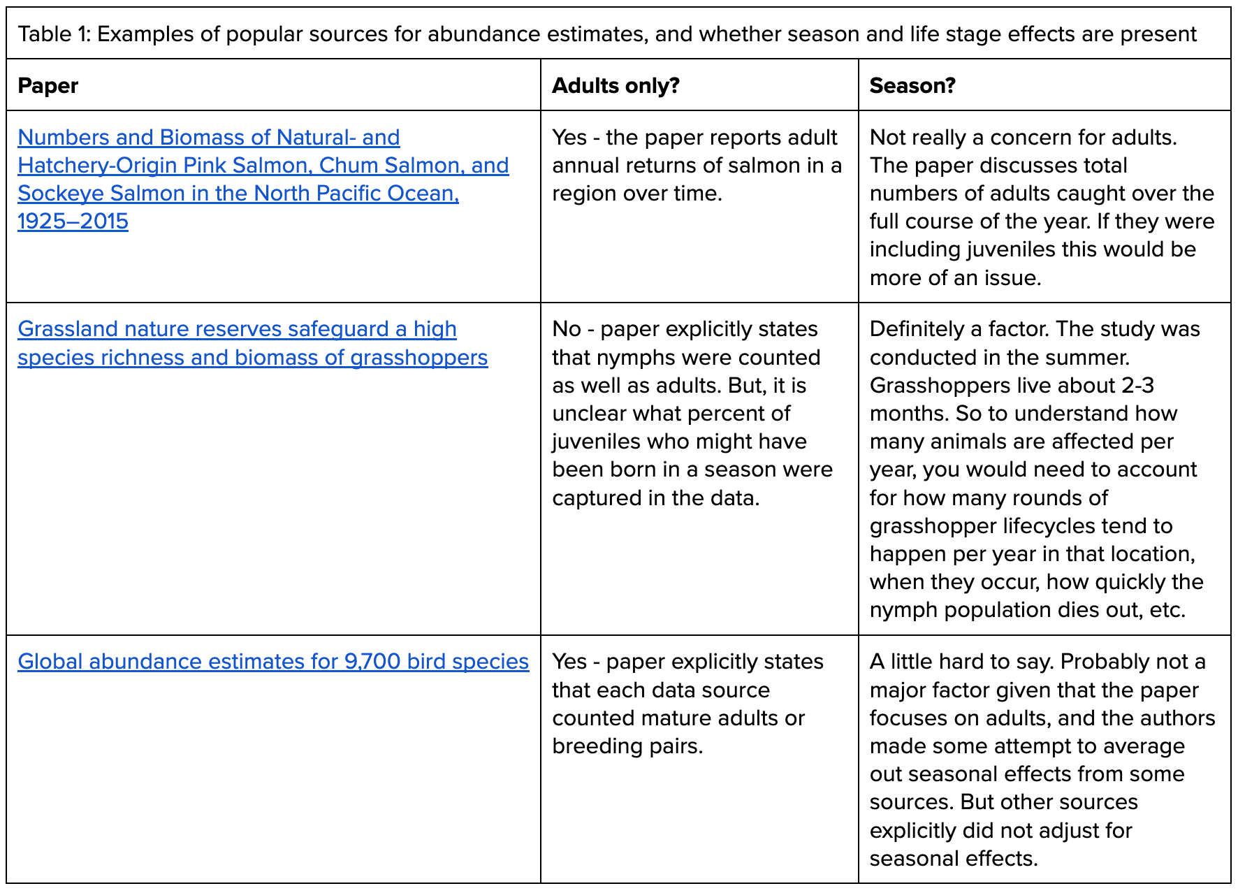
To illustrate the actual effect of excluding juveniles on the difference between “topline population estimate” and “actual number of individuals who existed in a given period,” we did a deeper analysis of a widely-cited estimate of global bird abundance.
Callaghan et al. 2021 — Global Bird Abundance
Global abundance estimates for 9,700 bird species is one of the most highly cited animal abundance estimates in the scientific literature. The authors’ median estimate is that there are 50.5 billion wild birds across 9,700 species (approximately 92% of extant bird species). Their mean estimate was 428 billion birds, so this estimate is highly imprecise. For the purposes of our analysis, we’ll use the 50.5B median figure.
To reach their median estimate, Callaghan et al. pull data from three sources: Partners in Flight, which estimates adult breeding populations; BirdLife, which estimates mature birds capable of reproduction; and BTO, which estimates breeding pairs (which the authors converted to individuals). They used these datasets and eBird data to estimate species-specific densities of 724 well-studied species. Then they used habitat and range data to scale this up into abundance estimates for around 9,000 other species. This was obviously error-prone, and the output was a very broad range.
We can imagine an animal welfare advocate considering an intervention that improves the lives of birds, or reduces the painfulness of their deaths. They might naively estimate days of experience by multiplying their topline 50.5B estimate by 365 (18.25T bird-days experienced), and calculate deaths by dividing this figure by the average annual mortality rate of adult birds (~0.4, so ~20B deaths). So, we have our naive welfare-relevant figures — 18.25T bird-days, and 20B potentially painful deaths.
To compare this naive estimate to a more accurate one, we can look at Callaghan et al’s taxonomic order-specific breakdowns, and then find estimates of juvenile mortality and lifespan for each order. To calculate this, we looked at the hatchling (e.g., juvenile birds in the nest), 1 year, and adult mortality rates by bird order, along with the average age of birds when they begin breeding. We made a variety of simplifying assumptions (namely assuming that all birds within an order have similar life histories, etc), but overall, the model should still be useful. Some data are assumed based on similar birds, though given that most birds are Passeriformes, shorebirds, and gulls, these assumptions would not change the topline results substantially if better data were found.
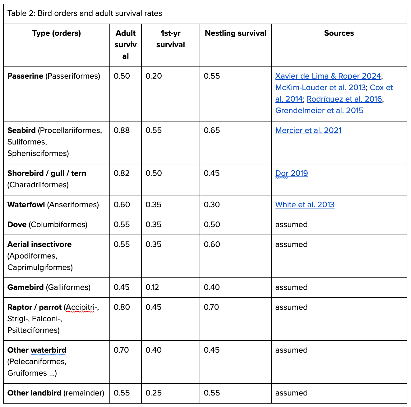
Once we take into account these figures, we can estimate both the total number of deaths likely to occur in a year, and the total individual-days experienced annually:
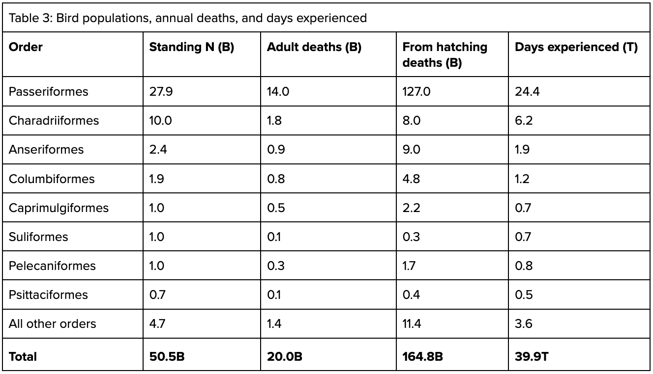
So, in a given year, to maintain a stable 50.5B population, 164.8B deaths might occur (8.24x our naive estimate), and 39.9T days of experience might occur (2.19x our naive estimate). The stable population estimate is therefore missing the welfare-relevant mark by several times.
Comparing five example groups of animals
A 2x error might not be a major issue, given the already highly uncertain nature of most wild animal interventions. But for arthropods and other highly r-selected fauna, the difference can be more extreme. To show the variation between taxa, we created toy models of 5 groups of animals with very different reproductive and survival strategies:
Passeriforme birds, the most common birds
North Atlantic Salmon, a highly r-selected fish
Grasshoppers, a mildly r-selected insect suborder
Ants, a relatively k-selected insect family
Aphids, a highly r-selected insect family
To do this, we used estimates of juvenile mortality, life expectancy at birth and different developmental stages, and Little’s law to estimate how many deaths occur annually in a population, and how many days are experienced by the population in an average year. Our methods are outlined in Appendix A.
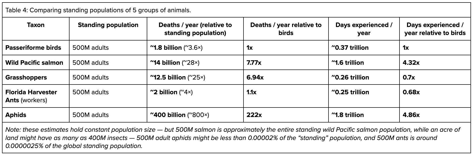
While these figures should not be taken as exact (given the large variety of animals we’ve collapsed into single rows, and that some of these animals, like aphids, will rapidly grow in population then crash), this exercise produces interesting results:
Among these five groups of animals, insects sit at both extremes:
Perhaps most surprisingly, the model ants face similar numbers of annual deaths per year for a given population size compared to the model birds. Because they have fairly intensive rearing practices (e.g., having specialized roles like nurses) ant mortality is relatively low at early life stages. And because they have shorter lifespans than birds, the result is also fewer days experienced.
On the other end of the spectrum are the model aphids. Aphids can reproduce both sexually and asexually, and have fairly extreme reproductive traits. For example, sometimes new aphids are born already pregnant with the next generation, and asexual reproduction can carry an aphid population for 10-30 generations prior to the next round of sexual reproduction. Populations are able to double weekly. The net result is that, in our model, to maintain a stable 500M population, 222x as many aphid deaths would have to occur, and in aggregate the aphids would live for 4.86x as many animal-days as birds at the same population size, despite their short average lifespan.
Of course, there are also vastly more insects than vertebrates — the standing population of ants may be as high as 20 quadrillion, while 500M adults is approximately the entire wild Pacific salmon adult population — so the ceiling for insects affected by a given intervention could be higher regardless of throughput differences. But as many interventions don’t reach their ceiling, the specifics of the intervention are more important than generic comparisons.
Animals as diverse as grasshoppers and salmon might face similar numbers of deaths per year (over 6x the birds) for a given population size, but very different numbers of days experienced (due to the salmon’s much longer lifespans). In contrast, aphids and salmon have more similar “days experienced” in a given population size while the aphids have a far higher number of deaths.
Whether it makes sense to prioritize a given population of grasshoppers, salmon, or aphids would therefore depend in part on whether the available interventions influence some percentage of lifespan, vs a specific experience that every individual goes through.
Implications for impact estimates
As we’ve shown, impact estimators need to examine more than just topline population estimates to calculate the possible impact of a potential intervention. They need to consider how the estimate was constructed, and incorporate information about the life history of the species in question. But, critically, we must also consider what life stages the intervention is likely to affect.
If we recommend putting out water to reduce the risk of dehydration for birds in the winter, we need to consider only those animals who have left the nest. But if we’re reducing the incidence of some disease, nestlings would need to be included. Essentially, interventions affecting mature adults will often affect a more similar number of individuals to literature population size estimates (especially for vertebrates), while those affecting juveniles are the ones that are most undercounted by naive estimates.
All of the foregoing discussion roughly assumes we’re talking about animals with fairly stable populations. If the population in question is not stable over the period you expect your intervention to be active, that will also change the number of individuals affected. On the flip side, even if the adult population is stable, various interventions may still alter the number of individuals that live and die, or are otherwise affected. For example, if we increase the number of egg predators while decreasing the number of non-egg-stage predators, these changes could balance out such that the impact on average adult population size is minimal. But the number of existing individuals overall could change dramatically, as many fewer eggs hatch and more of the juveniles that are born survive.
Finally, interventions will usually operate regionally rather than globally, with few exceptions. So global estimates might not actually be the best way to estimate who will be affected by an intervention, or to compare the promise of interventions. Nevertheless, to the extent it’s ever useful to present information about the total size of wild animal populations, it should be kept in mind that the numbers are potentially much bigger than what is shown, depending on the source. Arguments for focusing on a specific species on the basis of stable population size are generally not justified, because species with the same stable population sizes can include vastly different numbers of days of experience and total individuals lived. Impact estimators should endeavor to make more careful estimates of SADs and DALYs using an appropriately created estimate of the actual individuals affected.
Takeaways
To summarize the points from above:
You can’t naively multiply “the welfare cost of some event lasting time X years” times “average number of individuals” and get a reasonable estimate of the animal-years of effect.
Unless an intervention affects a stable population of reproductive adults only, many literature estimates will undercount the number of individuals affected, especially for highly r-selected species.
Species priority might change for interventions that improve environmental conditions vs interventions that improve the painfulness of death or the quality of another universal experience (like the first few moments of life).
To correct population estimates to get a better idea of the number of individuals affected by an intervention, you need (at minimum) to understand how the underlying estimate was generated, and account for juveniles, seasonality, shifting stable sizes. You also need to think carefully about what life stage your intervention is actually likely to target.
There are also some implications of this for future research, and others working within the wild animal welfare sciences.
It might be worth exploring if ecological motivations can justify better research into arthropod life history, and not just studies of stable adults and other conservation-relevant metrics. Ecology has significantly more funding and talent than wild animal welfare, so if the things we care about estimating are only relevant to animal advocates, it will be harder to get relevant research funded.
If wild animal advocates develop their own tools for making population size estimates, they need to ensure juveniles are included, and present data broken down by life stage.
We shouldn’t assume that research on the most numerous populations (based on topline estimates) are always the highest priority. Because of the pattern of trade-off between lifespan and numerosity, interventions that affect entire lifespans can be more impactful in longer-lived (but still numerous) animals than those that are even more r-selected but have extremely higher, earlier juvenile mortality.
When researching cascade effects or trying to find interventions that don’t change population sizes, age dynamics need to be considered. Environmental and management shifts that change age dynamics will alter the number of individuals alive and days experienced each year, even when the stable population size isn’t expected to change. This means that shifts between predators that focus on different life stages matter, changes between diseases that affect different life stages matter, etc.
Appendix A: Methodology for animal throughput estimates
We estimated two welfare-relevant annual flows, deaths per year and individual-days experienced per year, across salmon, passerine birds, grasshoppers, Florida harvester ants, and aphids, then normalising each to 500 M standing adults. There are lots of caveats with this work — in particular, in some places, we’re inferring from other species what survival rates, etc. may look like. For ants, we chose a specific example species, due to the high level of variability in lifespan across species (the other animals we looked at have more homogenous life histories across species). These models are massive oversimplifications and shouldn't be taken too literally.
Common framework
Deaths/yr and days/yr are estimated from a “born” boundary which is set to an animal’s first post-hatch / post-birth juvenile stage (salmon fry, bird hatchling, grasshopper/aphid nymph, ant larva). Egg and pre-hatch stages are excluded.
Steady state (births = deaths): deaths/yr (all stages) = births/yr at born boundary = B; adult recruitment/yr = adult deaths/yr.
Little’s Law: days/yr = adult-days + survivor-juvenile-days + non-survivor-juvenile-days; mean age at death = days/yr ÷ B.
Adult reference A = 500 M. Iteroparous (birds, ants, aphids): standing stock, adult deaths/yr = A ÷ adult-lifespan. Semelparous (salmon; univoltine grasshoppers): A = annual adult cohort, adult deaths/yr = A.
Wild pacific salmon
Born boundary = fry. Semelparous → returns ≈ adult deaths. Mix of three species (chum, pink, and sockeye).
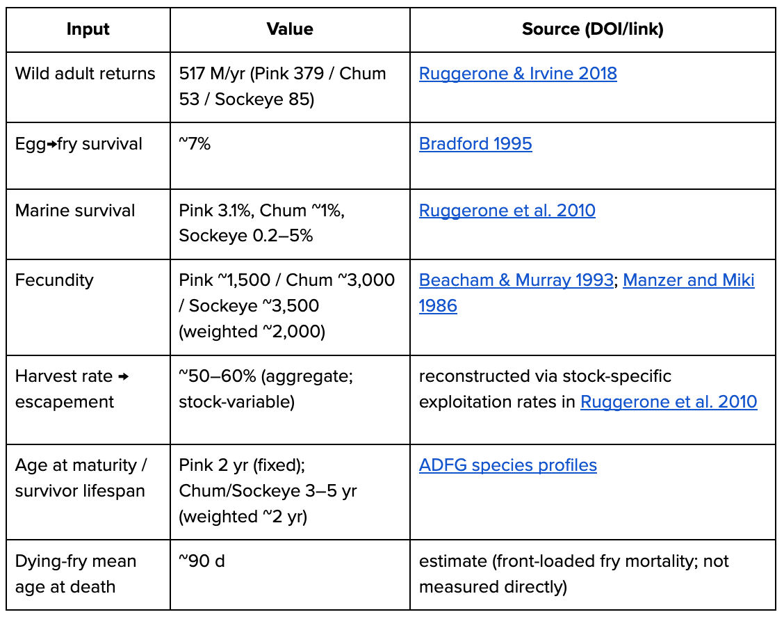
escapement E = 517M × (1 − ~0.6) ≈ 207M
fry B = E × 0.5 × ~2,000 × 0.07 ≈ 14.5B
deaths/yr = B ≈ 14B
days/yr = 517M×~730d + (B−517M)×~90d ≈ 1.6T fish-days
Passeriform birds
Born boundary = hatchling. Iteroparous. Great tit used as example species.
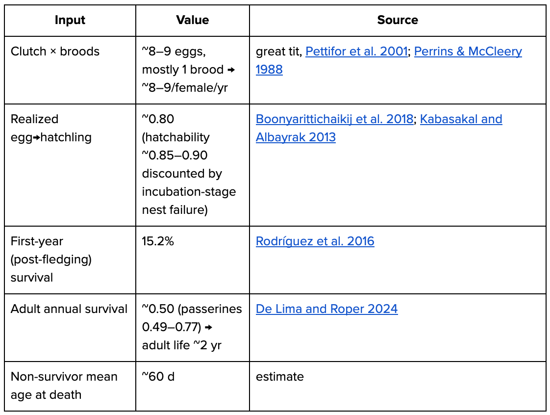
adult deaths/yr = 500M × (1 − 0.50) = 250M
hatchlings/yr B = 250M females × ~9 × 0.80 ≈ 1.8B   (~3.6× adults)
deaths/yr = B ≈ 1.8B
days/yr = 500M×365 + 250M×365 + (B−250M)×60d ≈ 0.37T
Grasshoppers
Born boundary = hatchling nymph. Univoltine. Central-European grassland Orthoptera used as example species.
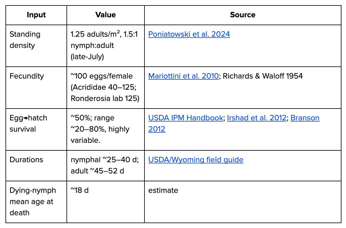
hatchlings/m² = 1.25 × 0.5 × 100 × 0.5 ≈ 31
deaths/500M ≈ 12.5B
days/m² = 1.25×45 + 1.25×40 + 30×18 ≈ 647 → 517/adult;
days/500M ≈ 0.26T
Ants
Born boundary = larva. “Adults” = sterile workers. Pogonomyrmex badius (Florida harvester ant) used as example species.
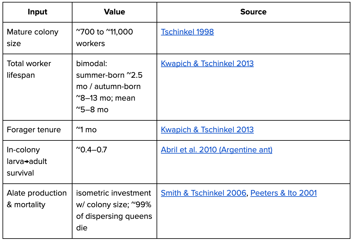
worker deaths/yr = 500M ÷ ~0.5–0.67 yr ≈ 0.75–1.0 B
larvae born/yr = worker recruitment ÷ larva→adult(~0.4–0.7) ≈ 1.1–2.5 B   (= worker-line deaths)
+ reproductive brood (alates, ~all die) ≈ 0.2–0.5 B
deaths/yr (all stages, born = larva) ≈ 1.5–2.5 B
days/yr = 500M×365 (workers) + brood-days ≈ 0.25 T (~500/worker; turnover-independent)
Aphids (asexual summer phase)
Born boundary = live-born nymph (viviparous — no egg stage). Multivoltine; asexual phase means all-female and replacement = 1 daughter/female. Based on data from several species.
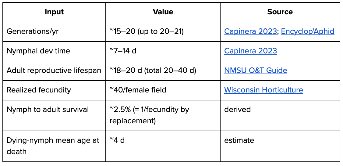
adults through/yr = 500M × (365 ÷ 18d) ≈ 10B;  nymphs born/yr B = 10B × 40 ≈ 400B
deaths/yr = B ≈ 400B;  days/yr = 500M×365 + 10B×7d + 390B×~4d ≈ 1.8T